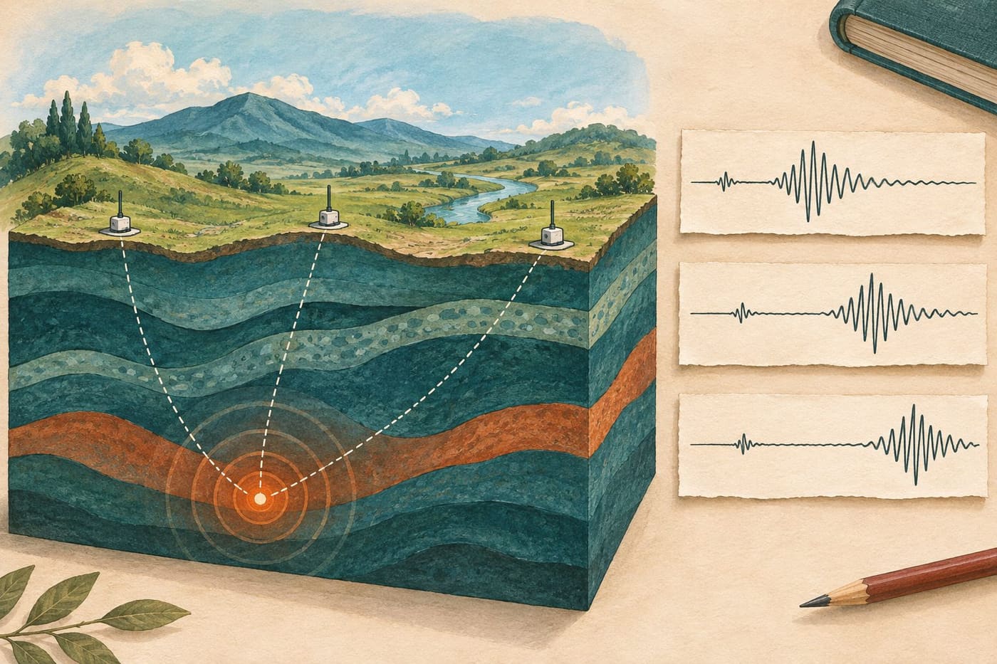
A line on a seismic display suddenly becomes busy. It is tempting to treat that shape as a complete description of an earthquake: where it happened, how large it was and what people nearby experienced. A seismogram is more specific. It records a signal at a particular instrument, with a particular time scale and measurement channel. The scientific interpretation comes from connecting that record with other observations and a model of how waves travel.
This guide explains that connection through original classroom examples. It is not an analysis of a current earthquake, an earthquake prediction or an emergency bulletin. The invented station times below are arithmetic exercises, not observations submitted to a monitoring network. The aim is to understand what a trace contributes to a location estimate and what additional information the estimate requires.
Identify the record before interpreting its shape
The British Geological Survey's introduction to earthquake detection distinguishes the measuring instrument from the seismogram it produces. It explains that modern instruments convert vibration into electrical signals and can measure motion in three directions. A trace is therefore not simply a photograph of a crack moving underground.
Before examining a screenshot, find its station, channel, date, time convention and scale. If any of these are missing, retain that limitation in your notes. A cropped image may be attractive in a presentation while removing the very information needed to compare it with another record.
Imagine two students receive the same trace. One labels it “the earthquake”; the other labels it “the north-south channel at the fictional Cedar station during the stated interval.” The second description is less dramatic but more useful. It tells a later reader what the image actually represents and leaves room for other stations to record different signals from the same event.
Keep an unmarked copy of a classroom record alongside your annotated copy. Marking a suspected arrival is an interpretation. Preserving the original makes it possible to discuss why that mark was placed there, instead of letting a coloured arrow become indistinguishable from the underlying data.
Learn the display's time convention
The USGS page About the Seismograms explains its Northern California drum-style displays. On that particular display, time runs across each row and continues on the next; a row represents fifteen minutes. Alternating colours help distinguish rows, rather than identifying a different earthquake type. The page also explains that magnification and background noise affect the appearance, and that vibrations or interference need not originate from earthquakes.
Those details belong to that display. Do not assume that every public seismic image uses fifteen-minute rows, the same colours or the same time labels. Read the documentation attached to the record you have chosen. A display format is a way of arranging measurements, not a universal scientific scale.
For an original paper exercise, draw a trace across two rows and put a labelled minute boundary between them. Place a marked arrival just before the boundary and another just after it. Ask a reader to calculate the elapsed time. The exercise exposes a simple mistake: treating the left edge of the second row as a new, unrelated event rather than a continuation.
If two screenshots use different clock conventions, convert the labels explicitly before comparing them. Write both the original label and the converted value. Otherwise, a clerical mismatch can look like a surprising physical delay. The quality of a scientific comparison begins with knowing what its axes mean.
Separate arrival time from the time the source began
BGS explains that P waves travel faster than S waves through the relevant solid material and that arrival times at different stations help locate an earthquake. The gap between identified P and S arrivals can provide a distance estimate using an appropriate travel-time relationship. This is the useful principle behind many classroom location exercises.
Consider a deliberately simplified model with a single path of length 72 kilometres. Assign a P-wave speed of 6 kilometres per second and an S-wave speed of 3 kilometres per second. These are chosen model values, not a description of the Earth's complete structure or an operational location formula.
In this model, the P travel time is 72 divided by 6, or 12 seconds. The S travel time is 72 divided by 3, or 24 seconds. If the source begins at the model clock's zero, the arrivals occur at 12 and 24 seconds, giving a twelve-second gap. Shift the source start to 100 seconds and the arrivals become 112 and 124 seconds. The gap stays twelve seconds.
That subtraction is the lesson. An arrival is recorded at the station after travel has occurred. It is not automatically the origin time. Comparing two arrivals can remove the common source-start time in this simplified setup, but the conversion from their gap to distance still depends on the assumed wave speeds and paths.
Use the arithmetic without mistaking it for the Earth
For our constant-speed model, the arrival-time difference equals distance multiplied by the difference between the reciprocals of the two speeds. With the selected values, that is distance multiplied by one-sixth of a second per kilometre. A twelve-second difference therefore corresponds to 72 kilometres in this model.
Now change only the model speeds to 5 and 3 kilometres per second while retaining a twelve-second gap. The reciprocal difference becomes two-fifteenths of a second per kilometre, giving 90 kilometres. The observed interval has not changed; the assumptions used to interpret it have. These numbers are a teaching comparison, not two competing estimates for a real event.
A useful worksheet keeps three columns: what was measured or stipulated, what was assumed, and what was calculated. Put the arrival gap in the first, speeds in the second and distance in the third. This prevents an assumed speed from quietly becoming an observation and prevents a calculated distance from acquiring more certainty than its inputs.
Do not use this toy arithmetic to locate a real earthquake from an online screenshot. Its value is explanatory: it shows why a travel-time model matters. Actual location work must deal with a three-dimensional Earth and information that the simple exercise deliberately leaves out.
Ask what one distance leaves unresolved
Suppose a flat classroom map shows a station at its centre and the exercise supplies a distance of five grid units. Many points satisfy that distance. Draw the circle: the information restricts the possible position but does not select one direction around the station.
Add a second fictional station with its own distance circle. The circles may intersect at two places. A third appropriately placed station can resolve the simple map exercise. BGS uses a three-station circle illustration to explain this principle. The map is an introductory model; it is not a claim that operational earthquake location consists only of drawing three perfect circles.
Try the exercise twice. First, choose distances that meet at one clean point. Then slightly change one radius. The second set may fail to meet exactly. Instead of forcing the circles to intersect with a thicker pencil, ask which pieces of information are uncertain and what kind of best-fitting answer would be reasonable.
The exercise also makes a useful distinction between a station and a source. A station is where the record was made. A source location is inferred using records and assumptions. A screenshot labelled with a town containing a station does not, by that label alone, establish that the earthquake occurred beneath that town.
Understand a location as a fitted solution
The USGS explanation of locating earthquakes describes estimating location, depth and origin time together. A candidate source and a model of seismic velocities predict arrival times at the stations. Those predictions are compared with the observed times, and the candidate is adjusted to improve the fit. Its account describes an iterative least-squares approach.
To understand the comparison without solving a real event, make a fictional three-row table. Let observed arrivals be 20, 25 and 31 seconds, and one model's predicted arrivals be 19, 27 and 30 seconds. Subtract prediction from observation. The residuals are plus one, minus two and plus one second. Their squared values sum to six square seconds.
A second invented model predicts 20, 26 and 30 seconds. Its residuals are zero, minus one and plus one, whose squared values sum to two. Under this deliberately limited comparison, the second set fits these three arrival times better. That does not establish that the second model is a valid physical earthquake solution; the exercise compares only a numerical measure of fit.
Why square the differences in this example? Adding the first model's signed residuals gives zero, concealing the discrepancies. Squaring keeps positive and negative errors from cancelling. The arithmetic offers a concrete way to understand the word “fit” without pretending that a classroom table replaces the full scientific calculation.
Keep depth distinct from the point on the map
The epicentre is the surface point above the earthquake's starting location, while the hypocentre is the location at depth. A two-dimensional map cannot by itself display every part of that three-dimensional relationship. A pin is convenient for navigation, but it should not erase the depth information attached to an event record.
The USGS's explanation of depth determination discusses identifiable reflected phases such as pP and their timing relative to P. Their travel-time relationship can provide depth information. This illustrates why specialists examine more than the biggest peak in a waveform.
For a classroom comparison, imagine two source points directly beneath the same surface grid position but at different depths. They share a surface projection, yet they are not the same three-dimensional location. Label both coordinates and depth in the diagram. The point is conceptual; no real travel times or shaking consequences follow from the sketch without further information.
When reading a catalogue, preserve the depth value and any stated qualification alongside the map position. If a source does not provide the uncertainty you need, say so. Adding decimal places to a copied coordinate does not supply new measurements or make the underlying estimate more precise.
Distinguish absolute position from relative pattern
A USGS Yellowstone Volcano Observatory article on precise relative earthquake locations explains how uncertainties in wave speeds and picked arrival times affect ordinary location estimates. Nearby events can be analysed together to improve their positions relative to one another. The article distinguishes a group's internal arrangement from its exact overall placement.
Think of an original drawing exercise with five dots on a transparent sheet. You can measure the separations among the dots carefully while remaining uncertain about where the whole sheet belongs on a base map. Moving the sheet changes absolute positions but preserves the pattern within it. This is an analogy about reference frames, not a physical model of a fault.
That distinction helps when two maps show a similar group with different amounts of apparent scatter. Ask whether the maps use different methods, different event selections or different coordinate treatments. Do not immediately interpret every shift in plotted dots as movement of the rock between the map publication dates.
The scientific result may concern a pattern resolved through improved analysis. To describe it accurately, retain the method and scope of the comparison. “The revised analysis resolves a tighter arrangement” and “the earthquakes physically moved” are very different claims.
Write a caption that keeps observation and inference together
A responsible caption can be brief while retaining the essentials. For the classroom examples here, a suitable caption would identify the fictional station, model clock, marked arrivals and chosen constant speeds, then state that the distance is calculated within a simplified exercise. It would not label the diagram as a live earthquake record.
For a real published figure, use the actual source's station information and caption. Identify whether you are showing raw records, processed traces, a catalogue map or an explanatory illustration. If the source does not support a claim about magnitude, damage or prediction, do not add that claim because the figure looks dramatic.
Magnitude and local shaking answer different questions from the timing exercise developed here. The USGS overview of magnitude, energy and intensity explains those distinctions. Our separate Chiba earthquake bulletin guide discusses reading event-report fields; this article concentrates on how station records contribute to locating the source.
Read the trace as evidence with context
Begin with the station and axes, identify what the plotted signal represents, and keep recorded arrival times separate from source time. Then ask how multiple records and a travel-time model support the inferred position. The arithmetic examples show why assumptions, residuals and reference frames belong in the explanation.
An arrival mark needs a time scale; a calculated position needs a model and supporting records. You can appreciate the scientific work without turning one striking image into a complete event diagnosis. The useful result is a clearer account of what was recorded, what was assumed and what was inferred from their combination.
Sources and review scope
Sources consulted 18 November 2026. Primary educational explanations from the British Geological Survey and USGS support the instrument, wave-arrival and location-method discussion. All numerical exercises and paper-map examples are original hypothetical models. No live seismic data were analysed, no felt report was submitted and no current earthquake or future hazard was predicted.
- BGS: How earthquakes are detected, located and measured
- USGS: About the seismograms
- USGS: How seismologists locate an earthquake
- USGS: Determining earthquake depth
- USGS: Precise relative earthquake locations
- USGS: Magnitude, energy release and intensity